The spreadsheet module is at best a weak imitation of Microsoft Excel, and Microsoft has shown no interest in updating it since version 4.x which was initially released in 1995- despite new releases having much later version numbers, there have really been no changes or improvements of substance since that time.
If you are using Microsoft Works spreadsheet, my recommendation:
1) Open any important spreadsheets that you've made using MS Works, use the File/Save As menu, and save in Excel (*.XLS) format.
2) Download and install the free, open source LibreOffice.org office suite -- it include a spreadsheet compatible with Excel spreadsheets, along with a good, MS Word compatible word processor, and a good MS PowerPoint-compatible presentation program.
3) You may want to set LibreOffice to save in Excel format by default, making it easier to share your spreadsheets with other people. (I have a tutorial on configuring OpenOffice.org at: http://www.zisman.ca/OOSetup/)
Nevertheless, the content of this tutorial may prove useful as an introduction to spreadsheets in general, whether you are using Microsoft Works, AppleWorks, Excel, OpenOffice.org, or whatever.
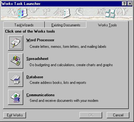
Spreadsheets are popular computer application for working with numbers. Some popular spreadsheets are Microsoft Excel and Lotus 1-2-3. Microsoft Works also includes a spreadsheet-- similar but less complex than Excel. To open a spreadsheet in Works 4.5,chooseFile/New and click on the Spreadsheet button (You may have to click on the Works Tools tab. Note that the opening screens will look different in both older versions of Works and Works 2000 or newer-- my samples are from Works 4.x. The rest of this tutorial will be fairly similar across versions).

You’ll see something like this:
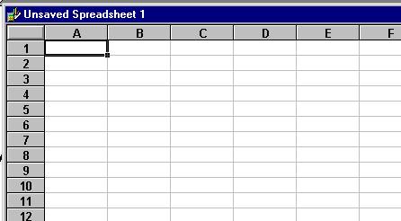
The letters along the top identify columns-- which go up and down.
We might speak of column C, After the first 26, columns are labeled AA, AB, AC, etc.
The numbers along the side identify rows-- which go across.
A single rectangle is called a cell and has an address made up of its column and row-- A3, D11, CF123, etc.
We enter information into cells-- which is different from a word processor. For example, when you center text, it is centered in its cell, not across the page. You select a cell by clicking on it.
You can select an entire column by clicking on the letter at the top of the column-- or select an entire row by clicking on the number at the left of the row.
A rectangular group of cells is referred to as a range. You can select a range by holding your (left) mouse button down while moving across the range, or by clicking in the top-left corner, holding down the shift-key and clicking in the bottom-right corner of the range. Notice that the first cell in the range isn’t highlighted-- a source of endless confusion!
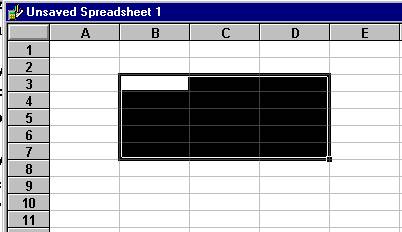
A range is referred to by the top-left and bottom-right cells, with a colon in between-- B3:D7
You can type a number of things into a cell:
-- labels are words, phone numbers, etc.
-- numbers are (duh!) numerical data (note that phone numbers aren’t numbers)
-- formulas perform calculations on numbers-- when you’re done typing a formula, it only shows the answer. to see the formula that you typed, look in the formula bar above the spreadsheet:
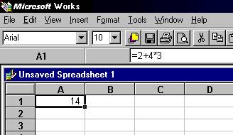
Note the labels, numbers, and how the answer appeared in cell B6, while the obscure-looking formula that I typed in that cell shows up above.
To get the total amount of rainfall in the three months listed above (instead of the average), we could type a number of formulas in cell B6. Note that all formulas start with an equal sign (that’s how the spreadsheet knows it’s a formula!):
= 25 + 17 + 44 <-- simply adds the three numbers = B3 + B4 + B5 <-- adds whatever numbers are in those 3 cells =sum(B3:B5) <-- gets the sum of all the numbers in the rangeThe later is most useful-- especially if you need to add a large number of cells. Because you’re referencing the cell addresses, if the number in a cell changes, the answer automatically changes as well.
Arithmetic with spreadsheets :
| Addition: | =15 + 30 | =B3 + D7 |
| Subtraction: | = 30-15 | =B3 - D7 |
| Multiplication: | = 30 * 15 | =B3 * D7 |
| Division: | = 30/15 | =B3/D7 |
| Exponent: | = 30^2 | =B3^2 |
| Square Root: | =sqrt(16) | =sqrt(B3) |
You can mix numbers and cell addresses: =B7 + 3 for example.
And you can combine different arithmetic operations, using parentheses as needed:
=B7 * (A3+A18 - 47)
By nesting parentheses, you can make very complex arithmetic sentences-- but most of us won't ever need to do this!
A function is a formula built-into the spreadsheet. functions are applied to whatever is inside the parentheses. Typical spreadsheets have 50-200 built-in functions, for business purposes (mortgage calculations, for example), statistical analysis, and other specialized purposes. Two are most often used by ‘everyday’ people:
=Sum to add all the numbers in a range: =sum(A5:D15) =Avg to get the average of all the numbers in a range: =avg(A5:D15)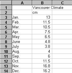
-- (data is from Vancouver Tourism’s website: http://www.vancouvertourist.com/ )
A couple of tricks!
-- When you start typing the title in cell B1, notice that all the words fit-- even though the cell is too narrow to hold them all. They ‘spill out’ into the cells to the right-- but the text is actually all in cell B1.
-- Type the word ‘January’ in cell A3, but don’t type the other months. instead, select that cell, and a bunch of cells underneath-- highlighting cells A3 to A14.
From the Edit Menu, click on ‘Fill Series’, and click on Month:
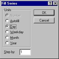
It will type in all the months automatically. This is also good if you have a numerical series-- 1, 3, 5, etc. or even 1, 2, 3, 4, .
-- You can adjust the look of your sheet. to make columns wider or narrower, click on the border between the two letters at the top of the column. when your mouse pointer changes to a double-headed arrow:
you can drag the border to the left or the right.
You can click on the on letter or number tab on top (or on the right) of a column or row to select the entire column or row-- and change the font, size, style of anything in the column. or click on the left-align, right-align, or center-align buttons to line up the text in that column. or on the $ button to make any numbers formatted as currency:
![]()
(Back to work on our Vancouver Climate worksheet):
After you’ve entered the labels and numbers for the 12 months, type the words:
Total in cell A15
Average in cell A16
=sum(B3:B14) in cell B15
=avg(B3:B14) in cell B16
Bingo-- you’ve got the answers. Notice how the average displays to 6 decimals-- probably more than you want! To change it, select that cell,
Click on cell B16, then click on the Format menu, then on Number. select Fixed, and enter the number of decimal places desired (perhaps ‘0’).
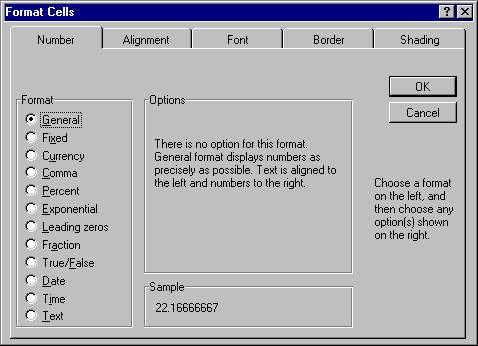
This Format/Number menu lets you display numbers as currency, percent, and other useful formats, as well as control the number of decimal places displayed-- it doesn’t change the answer, only the way it shows the answer (hint-- it rounds off to the desired number of decimal places).
. is spreadsheet jargon for making a graph from your data. Note that we need to enter the data first, but then, the spreadsheet can automatically make a graph, which will change if your data changes.
With your Vancouver Rainfall data, highlight the range A3:B14, and click on the Tools menu, then on Create New Chart. you should see:
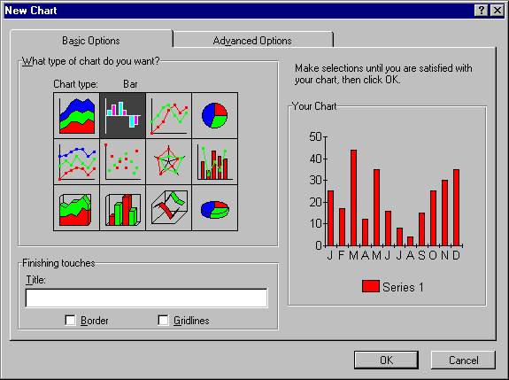
It instantly shows your data in a bar-graph. you can click on the different chart types to see how your chart will look-- add a title, border, gridlines, etc. and preview how it will look. Make selections that you like, and click OK.
-- Note that different types of data lend themselves to different chart types. This data might work as a pie chart, for instance, showing more graphically the contribution of each month to the whole year’s rainfall.
-- You’ll notice that the data is labeled on your chart as ‘Series 1’, We can probably do better-- click on the Edit menu, then on Legend/Series Labels.
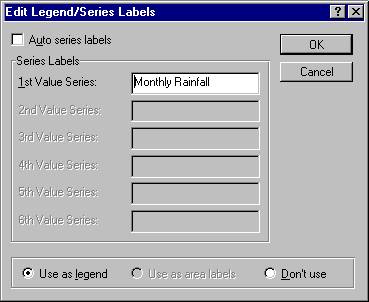
You’ll need to uncheck the [x] Auto Series Labels item in order to enter your own label for the data.
-- Using the various Charting Menu commands, you can ‘pretty up’ your chart some more. Check out:
- Edit/Title for the chart’s Title and Subtitle, and the titles for the X and Y axis
- Format/Shading & Colour or Font & Size
-- You can create multiple charts from the same data or different data on a single worksheet. a bar chart and a pie chart from the Rainfall data, for example. Use the Tools/Rename Chart or Tools/Delete Chart to help manage multiple charts.
-- The charts are saved along with the main spreadsheet. you don’t get separate File/Open or Save commands just for the charts. To return to the spreadsheet, use the View command.
You can make your chart more complex. Edit the spreadsheet, adding Average Temperature data:
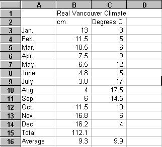
By selecting cells A3:C14, you can create a bar chart showing both rainfall and temperature!
-- You can enter data in the spreadsheet, select a range, Edit/Copy, then Paste it into your word processor for an instant table. You can use the spreadsheet to put a list of names into alphabetical order (select the list, then use the Tools menu’s Sort item to re-arrange it into alphabetical or numerical order), then copy it into your word processor if desired.
-- Similarly, after creating a chart, you can insert it into your word processor. With the chart showing, choose Edit/Copy, then go to your word processor and Edit/Paste. That’s how I got the chart shown above, for example.
-- You can use spreadsheets for lots of complex, repetitive tasks involving numbers. the work is in setting up the spreadsheet the first time (‘making a template’), after that you just enter the data, and the spreadsheet does the work. an example is calculating marks, or income taxes.
If you make a spreadsheet you want to use over and over again, create one with a small amount of ‘dummy’ data. make sure the formulas work as desired. For example, you could make one to calculate grades by adding up what all your assignments are out of, the adding up what each student actually got, then dividing what each student’s total by the ‘out-of’ total, formatting that answer as a percent.
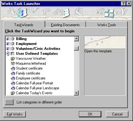
Save the template-- using the File/Save As command, and clicking on the Template button. Be careful not to check the ‘[ ] Use this template for new Spreadsheet documents’ option or it will pop up whenever you try to create a new spreadsheet.
To open the template, choose File/New, and click on the Task Wizards tab. scroll down the list to User-Defined Templates, and you’ll see yours.
Make a self-marking test
Here's a neat trick that works in the Works spreadsheet, Excel, and probably others. I got it from PC Magazine's helpful User-to-user column (http://www.pcmag.com).
This spreadsheet asks true/false, yes/no, or simple answer questions in Column A. Correct answers are contained next to the questions in Column B, but that column is hidden (or given a width of 0)-- the user types their answer into Column C.
In Column D, cells contain a formula such as =If(C2=B2,"Correct",""). Fill down or copy into each row with a question. If the user types the right answer, 'Correct' will appear; otherwise that cell will be blank.(Capitalization doesn't affect right answers).
Excel lets you count the number of correct answers using a formula like =countif(D1:D5,"Yes") (where the range D1:D5 is adjusted for the number of questions). That function doesn't work in Works 4.5 however.
To keep users from messing with the spreadsheet, in most spreadsheets, you can check the menus for a Protect item. in Works 4.5 however, this can only be set to protect the entires spreadsheet, which would make it impossible for users to enter their answers.